Learning Graph Matching through a Differentiable graph matching method based on Integer Linear Programming
This notebook is a follow up of the notebook called "a graph matching method based on the leading Eigen vector and Sinkhorn-Knopp algorithm"
This notebook shows how to perform graph matching thanks to Integer Linear Programming.
This notebook shows how to differentiate the solution of the graph matching thanks to finite difference method.
It is based on several papers and presentation :
- Puqing Chen, Romain Raveaux et al : Deep graph matching meets mixed-integer linear programming: Relax at your own risk ? CoRR abs/2108.00394 (2021)
Romain Raveaux: On the unification of the graph edit distance and graph matching problems. Pattern Recognit. Lett. 145: 240-246 (2021)
Romain Raveaux: PDF of a Talk on Differentiable Graph Matching meets Mixed-Integer Linear Program
Romain Raveaux: Video of a talk on Differentiable Graph Matching meets Mixed-Integer Linear Program
Authors : Romain Raveaux (romain.raveaux@univ-tours.fr), Puqing Chen (c.puqing@gmail.com)
Web site : http://romain.raveaux.free.fr
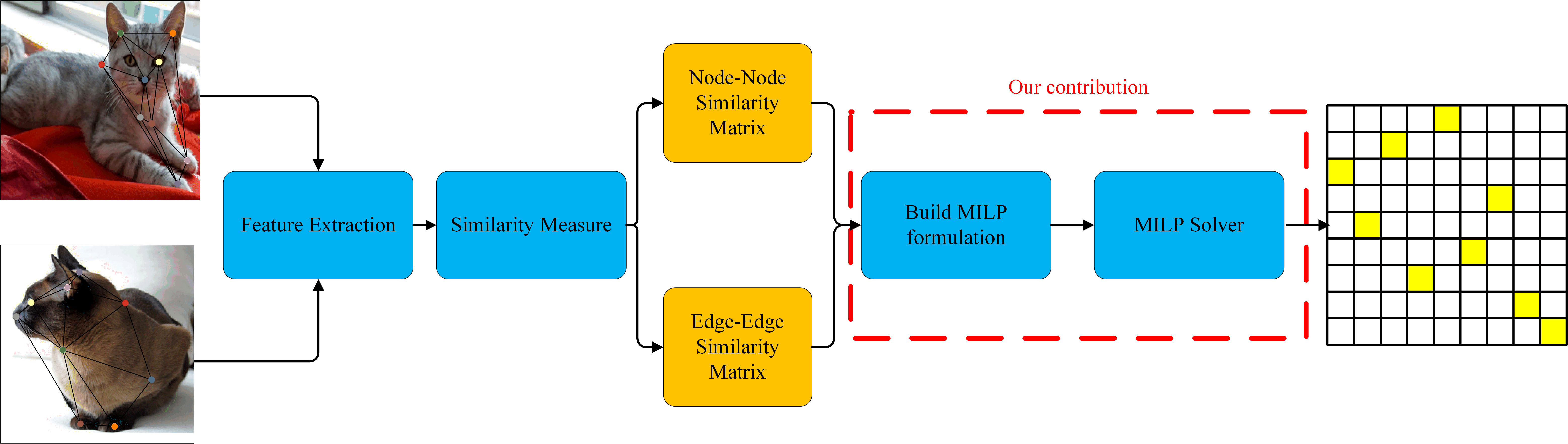
Global Architecture

from google.colab import drive
drive.mount('/content/drive')
The graph matching problem
The objective of graph matching is to find correspondences between two attributed graphs $G_1$ and $G_2$. A solution of graph matching is defined as a subset of possible correspondences $\mathcal{Y} \subseteq V_1 \times V_2$, represented by a binary assignment matrix $Y \in \{0,1 \}^{n1 \times n2}$, where $n1$ and $n2$ denote the number of nodes in $G_1$ and $G_2$, respectively. If $u_i \in V_1$ matches $v_k \in V_2$, then $Y_{i,k}=1$, and $Y_{i,k}=0$ otherwise. We denote by $y\in \{0,1 \}^{n1 . n2}$, a column-wise vectorized replica of $Y$. With this notation, graph matching problems can be expressed as finding the assignment vector $y^*$ that maximizes a score function $S(G_1, G_2, y)$ as follows:
\begin{align} y^* =& \underset{y} {\mathrm{argmax}} \quad S(G_1, G_2, y)\\ \text{subject to}\quad & y \in \{0, 1\}^{n1.n2} \\ &\sum_{i=1}^{n1} y_{i,k} \leq 1 \quad \forall k \in [1, \cdots, n2]\\ &\sum_{k=1}^{n2} y_{i,k} \leq 1 \quad \forall i \in [1, \cdots, n1] \end{align}
where equations \eqref{eq:subgmgmc},\eqref{eq:subgmgmd} induces the matching constraints, thus making $y$ an assignment vector.
The function $S(G_1, G_2, y)$ measures the similarity of graph attributes, and is typically decomposed into a first order dissimilarity function $s(u_i,v_k)$ for a node pair $u_{i} \in V_1$ and $v_k \in V_2$, and a second-order similarity function $s(e_{ij},e_{kl})$ for an edge pair $e_{ij} \in E_1$ and $e_{kl} \in E_2$. Thus, the objective function of graph matching is defined as: \begin{equation} \begin{aligned} S(G_1,G_2,y) =& \sum_{i=1}^{n1} \sum_{k=1}^{n2} s(u_i,v_k) \cdot y_{i,k} + \sum_{i=1}^{n1} \sum_{j=1}^{n1} \sum_{k=1}^{n2} \sum_{l=1}^{n2} s(e_{ij},e_{kl})\cdot y_{ik} \cdot y_{jl}\\ =& \sum_{i=1}^{n1} \sum_{j=1}^{n1} \sum_{k=1}^{n2} \sum_{l=1}^{n2} K_{ik,jl}\cdot y_{ik} \cdot y_{jl}\\ \quad \quad \quad \quad =&y^TKy \end{aligned} \end{equation}
Similarity functions are usually represented by a symmetric similarity matrix $K \in \mathbb{R}^{n1n2 \times n1n2}$. A non-diagonal element $K_{ik,jl} = s(e_{ij},e_{kl})$ contains the edge similarity and a diagonal term $K_{ik,ik} = s(u_i,v_k)$ represents the vertex similarity. $K$ is called an affinity matrix or compatibility matrix. In this representation, $K_{ij,kl}=0$ means an impossible matching or a very dissimilar matching. In essence, the score accumulates all the similarity values that are relevant to the assignment. The formulation in Problem \ref{model:iqpsubgm} is referred to as an integer quadratic programming. This integer quadratic programming expresses the quadratic assignment problem, which is known to be NP-hard.
Integer Linear Programming for Graph Matching
An Integer Linear Program (ILP) is a mathematical model where the objective function is a linear combination of the variables. The objective function is constrained by linear combinations of the variables. The Interger Linear Programming aims at solving the "exact" graph mathcing problem by exact we mean the not relaxed problem.
The entire formulation is called F2 see the reference for the full details and described as follows :

Where the function $c$ is a cost function defined as the opposite of the similarity function (c=-s).

Derivative/Gradient of the loss

Let's code !
- Read two graphs
- Extract features from graphs and images
- Compute the costs
- Implement the Interger Linear Program
- Compute the matching by solving the Interger Linear Program
- Differentiate the solution of the graph matching problem
- Train a Graph Neural NetWork + a Graph Matching Solver to solve a key point matching problem
!pip install networkx
Some imports : pytorch, matlplotlib, numpy and set your import directory
import numpy as np
import xml.etree.ElementTree as ET
import networkx as nx
import os
import matplotlib.pyplot as plt
import sys
import torch
homedir=""
sys.path.append(homedir) # go to parent dir
%matplotlib inline
Some more imports about gurobit
We will need a mathematical solver to solve the integer linear program representing the graph matching problem. We chose Gurobi to do so. Other mathematical solvers could be used such as Cplex ...
!pip install gurobipy # install gurobipy, if not already installed
Academic Licence
If you are a researcher or a teacher you can get an academic license. This will allow you to deal with larger instances.
import gurobipy as gp # import the installed package
# Create environment with WLS license
gpenv = gp.Env(empty=True)
gpenv.setParam('WLSACCESSID', 'wxxw')
gpenv.setParam('WLSSECRET', 'dff')
gpenv.setParam('LICENSEID',123)
gpenv.setParam('OutputFlag', 0)
gpenv.start()
# Create the model within the Gurobi environment
model = gp.Model(env=gpenv)
Download the data base of graphs.
We will use a part of the Pascal VOC data base for an illustration purpose.
https://paperswithcode.com/sota/graph-matching-on-pascal-voc
!wget "http://romain.raveaux.free.fr/document/voccar4tutopython.zip"
!unzip "voccar4tutopython.zip">lstfile.txt
Display an image
import matplotlib.pyplot as plt
data=plt.imread("voccar4tutopython/pair_10_1.png")
plt.figure(1)
plt.imshow(data)

Read a graph
Graphs are stored into XML files called GXL. Here is the way we parse them.
Each node has 4 attributes:
- x coordonate in the image
- y coordonte in the image
- p : angle to the normal
- gt : the id of the assigned node in the target graph
Each edge has 2 attributes:
- dist : distance between nodes in the spatial domain
- anglehorizon : an angle between the two nodes od the edge
def read_gxl(file):
"""Parse GXL file and returns a networkx graph
"""
tree_gxl = ET.parse(file)
root_gxl = tree_gxl.getroot()
node_position = {}
node_features={}
node_id = []
match={}
# Parse nodes
for i, node in enumerate(root_gxl.iter('node')):
node_id += [node.get('id')]
for attr in node.iter('attr'):
if (attr.get('name') == 'x'):
x = float(attr.find('Double').text)
elif (attr.get('name') == 'y'):
y = float(attr.find('Double').text)
elif (attr.get('name') == 'p'):
p = float(attr.find('Double').text)
elif (attr.get('name') == 'gt'):
gt = float(attr.find('Double').text)
match[i]=gt-1
node_position[i] = [x, y]
node_features[i]=[p]
node_id = np.array(node_id)
edgeattrs = {}
# Create adjacency matrix
am = np.zeros((len(node_id), len(node_id)))
for edge in root_gxl.iter('edge'):
s = np.where(node_id==edge.get('from'))[0][0]
t = np.where(node_id==edge.get('to'))[0][0]
for attr in edge.iter('attr'):
if (attr.get('name') == 'dist'):
dist = float(attr.find('Float').text)
elif (attr.get('name') == 'anglehorizon'):
anglehorizon = float(attr.find('Float').text)
# Undirected Graph
am[s,t] = 1
am[t,s] = 1
edgeattrs[(s,t)]=[dist,anglehorizon]
edgeattrs[(t,s)]=[dist,anglehorizon]
# Create the networkx graph
G = nx.from_numpy_matrix(am)
nx.set_node_attributes(G, node_position, 'position')
nx.set_node_attributes(G, node_features, 'p')
nx.set_edge_attributes(G, edgeattrs, "betweenness")
return G,match
G,match=read_gxl("voccar4tutopython/pair_10_1_0_.gxl")
Let us display the image and graph on it
print(G.nodes)
data=plt.imread("voccar4tutopython/pair_10_1.png")
nx.draw(G, pos=dict(G.nodes(data='position')),node_size=1)
plt.imshow(data)
plt.show()

G,match=read_gxl("voccar4tutopython/pair_1_1_0_.gxl")
data=plt.imread("voccar4tutopython/pair_1_1.png")
nx.draw(G, pos=dict(G.nodes(data='position')),node_size=1,edge_color='yellow')
plt.imshow(data)
plt.show()

Let us make a video with images and graphs
def draw(j):
ax.cla()
ax.axis('off')
ax.set_title('Image and Graph %d' % (j+1))
strgxl="voccar4tutopython/pair_"+str(j+1)+"_1_0_.gxl";
strimg="voccar4tutopython/pair_"+str(j+1)+"_1.png";
G,match=read_gxl(strgxl)
data=plt.imread(strimg)
nx.draw(G, pos=dict(G.nodes(data='position')),node_size=1,edge_color='yellow')
plt.imshow(data)
from matplotlib import animation, rc
from IPython.display import HTML
fig = plt.figure(dpi=150)
fig.clf()
ax = fig.subplots()
ani = animation.FuncAnimation(fig, draw, frames=30, interval=1000)
ani.save('GraphIMG.mp4')
HTML(ani.to_html5_video())
plt.figure(1)
G1,match1=read_gxl("voccar4tutopython/pair_1_1_0_.gxl")
data1=plt.imread("voccar4tutopython/pair_1_1.png")
nx.draw(G1, pos=dict(G1.nodes(data='position')),node_size=1,edge_color='yellow')
plt.imshow(data1)
plt.figure(2)
G2,match2=read_gxl("voccar4tutopython/pair_1_2_0_.gxl")
data2=plt.imread("voccar4tutopython/pair_1_2.png")
nx.draw(G2, pos=dict(G2.nodes(data='position')),node_size=1,edge_color='yellow')
plt.imshow(data2)

Let us draw the matching according to the matching ground truth
G1,match1=read_gxl("voccar4tutopython/pair_1_1_0_.gxl")
data1=plt.imread("voccar4tutopython/pair_1_1.png")
G2,match2=read_gxl("voccar4tutopython/pair_1_2_0_.gxl")
data2=plt.imread("voccar4tutopython/pair_1_2.png")
imall = np.zeros((500,1000,3))
imall[0:data1.shape[0],0:data1.shape[1]]=data1
xoffset=30
imall[0:data2.shape[0],xoffset+data1.shape[1]:xoffset+data1.shape[1]+data2.shape[1]]=data2
G1G2=nx.disjoint_union(G1,G2)
n1=len(G1.nodes())
for i in range(n1,G1G2.number_of_nodes()):
G1G2.nodes[i]['position']=[G1G2.nodes[i]['position'][0]+xoffset+data1.shape[1],G1G2.nodes[i]['position'][1]]
edgelista=[]
for i in range(n1):
k=match1[i]
edgelista.append((i, k+n1))
plt.figure(3)
nx.draw(G1G2, pos=dict(G1G2.nodes(data='position')),node_size=1,edge_color='yellow')
nx.draw(G1G2, pos=dict(G1G2.nodes(data='position')),edgelist=edgelista,width=1, alpha=0.5, node_size=1,edge_color='yellow')
#horizontal = np.concatenate((data1, data2), axis = 1)
plt.imshow(imall)
#plt.close()

Video of all the matchings
def draw(j):
ax.cla()
ax.axis('off')
ax.set_title('Image and Ground-Truthed Graph Matching for the pair %d' % (j+1))
strgxl1="voccar4tutopython/pair_"+str(j+1)+"_1_0_.gxl";
strimg1="voccar4tutopython/pair_"+str(j+1)+"_1.png";
strgxl2="voccar4tutopython/pair_"+str(j+1)+"_2_0_.gxl";
strimg2="voccar4tutopython/pair_"+str(j+1)+"_2.png";
#G,match=read_gxl(strgxl)
#data=plt.imread(strimg)
#nx.draw(G, pos=dict(G.nodes(data='position')),node_size=1,edge_color='yellow')
#plt.imshow(data)
G1,match1=read_gxl(strgxl1)
data1=plt.imread(strimg1)
G2,match2=read_gxl(strgxl2)
data2=plt.imread(strimg2)
imall = np.zeros((500,1000,3))
imall[0:data1.shape[0],0:data1.shape[1]]=data1
xoffset=30
imall[0:data2.shape[0],xoffset+data1.shape[1]:xoffset+data1.shape[1]+data2.shape[1]]=data2
G1G2=nx.disjoint_union(G1,G2)
n1=len(G1.nodes())
for i in range(n1,G1G2.number_of_nodes()):
G1G2.nodes[i]['position']=[G1G2.nodes[i]['position'][0]+xoffset+data1.shape[1],G1G2.nodes[i]['position'][1]]
edgelista=[]
for i in range(n1):
k=match1[i]
edgelista.append((i, k+n1))
# plt.figure(3)
nx.draw(G1G2, pos=dict(G1G2.nodes(data='position')),node_size=1,edge_color='yellow',ax=ax)
nx.draw(G1G2, pos=dict(G1G2.nodes(data='position')),edgelist=edgelista,width=1, alpha=0.5, node_size=1,edge_color='yellow',ax=ax)
plt.imshow(imall)
from matplotlib import animation, rc
from IPython.display import HTML
fig = plt.figure(dpi=150)
fig.clf()
ax = fig.subplots()
ani = animation.FuncAnimation(fig, draw, frames=30, interval=1000)
ani.save('GraphIMGMatching.mp4')
HTML(ani.to_html5_video())

Feature extractions from graphs and images
As mentioned before, graphs hols attributes on edges and nodes. In addition, we will add features based on the pixels of the images.
- For each node we will get an image patch centered on the node. The patch is then flatten to obtain a vector.
- For each edge, a features vector is obtained by making the difference between pixel features of the source and target nodes.
Node feature extraction and adjacency matrix
def ExtractNodeFeaturesFromImageAndAdjacencyMatrix(G,image):
nodelist, nodesfeatures1 = map(list, zip(*G.nodes(data='position')))
GnodesFeatures1 = np.array(nodesfeatures1)
GnodesFeatures1[:,:]/=GnodesFeatures1.max()
nodelist, nodesfeatures2 = map(list, zip(*G.nodes(data='p')))
GnodesFeatures2 = np.array(nodesfeatures2)
GnodesFeatures2[:,:]/=GnodesFeatures2.max()
GnodesFeatures = np.hstack((GnodesFeatures1, GnodesFeatures2))
boxsize=3
imagepad = np.pad(array=image, pad_width=[(boxsize, boxsize),(boxsize, boxsize),(0, 0)], mode='symmetric')
pixelfeatures= np.zeros((GnodesFeatures1.shape[0],(2*boxsize)*(2*boxsize)*3))
count=0
for (x,y) in nodesfeatures1:
xint=int(x)+boxsize
yint=int(y)+boxsize
pixelfeatures[count,]=imagepad[yint-boxsize:yint+boxsize,xint-boxsize:xint+boxsize].flatten()
count=count+1
pixelfeatures/=pixelfeatures.max()
GnodesFeatures =np.hstack((GnodesFeatures, pixelfeatures))
GadjacencyMatrix = np.array(nx.adjacency_matrix(G, nodelist=nodelist).todense())
#plt.figure(4)
#plt.imshow(imagepad)
#print(GnodesFeatures.shape)
#print(GnodesFeatures)
#print(Gadjacency)
return GnodesFeatures,GadjacencyMatrix
Extraction of the edge features + node features
def ExtractFeaturesFromImageAndAdjacencyMatrix(G,image):
GnodesFeatures,GadjacencyMatrix=ExtractNodeFeaturesFromImageAndAdjacencyMatrix(G,image)
indexedgessouce,indexedgesdest, edgesfeatures1 = map(list, zip(*G.edges(data='betweenness')))
edgesfeatures = np.array(edgesfeatures1)
edgesfeatures[:,0]=edgesfeatures[:,0]/edgesfeatures[:,0].max()
edgesfeatures[:,1]=edgesfeatures[:,1]/edgesfeatures[:,1].max()
EdgeList =np.zeros((len(indexedgessouce),2),dtype=np.int32)
EdgeList[:,0]=np.array(indexedgessouce,dtype=np.int32)
EdgeList[:,1]=np.array(indexedgesdest,dtype=np.int32)
node1sourcefeatures = GnodesFeatures[EdgeList[:,0],:]
node1destfeatures = GnodesFeatures[EdgeList[:,1],:]
Gedgesfeatures=node1sourcefeatures-node1destfeatures
edgesfeatures=np.hstack((edgesfeatures, Gedgesfeatures))
return torch.from_numpy(GnodesFeatures),torch.from_numpy(edgesfeatures),torch.from_numpy(GadjacencyMatrix),torch.from_numpy(EdgeList)
Some printing of the shapes of the features
strgxl1="voccar4tutopython/pair_"+str(1)+"_1_0_.gxl";
strimg1="voccar4tutopython/pair_"+str(1)+"_1.png";
G1,match1=read_gxl(strgxl1)
data1=plt.imread(strimg1)
print("Printing the first node")
print(G1.nodes[0])
print("Printing the edges : they have no attributes")
print(G1.edges)
print("Printing the nodes attributes")
print(G1.nodes(data='position'))
GnodesFeatures,Gedgesfeatures,GadjacencyMatrix,GEdgeList=ExtractFeaturesFromImageAndAdjacencyMatrix(G1,data1)
print(GnodesFeatures.shape)
print(Gedgesfeatures.shape)
plt.figure(6)
plt.imshow(data1)

def ComputeUnaryQuadraticCosts(G1nodesFeatures,G2nodesFeatures,G1edgesFeatures,G2edgesFeatures):
EdgeSimilarities = G1edgesFeatures.matmul(G2edgesFeatures.T)
QuadraticCosts=-EdgeSimilarities
NodeSimilarity=G1nodesFeatures.matmul(G2nodesFeatures.T)
UnaryCosts=-NodeSimilarity
return UnaryCosts,QuadraticCosts
Let us print the shapes of the unary costs and the quadratic costs
strgxl1="voccar4tutopython/pair_"+str(8)+"_1_0_.gxl";
strimg1="voccar4tutopython/pair_"+str(8)+"_1.png";
G1,match1=read_gxl(strgxl1)
data1=plt.imread(strimg1)
strgxl2="voccar4tutopython/pair_"+str(8)+"_2_0_.gxl";
strimg2="voccar4tutopython/pair_"+str(8)+"_2.png";
G2,match2=read_gxl(strgxl2)
data2=plt.imread(strimg2)
print(len(G1.nodes))
print(len(G1.edges))
print(len(G2.nodes))
print(len(G2.edges))
G1nodesFeatures,G1edgesfeatures,G1adjacencyMatrix,G1EdgeList=ExtractFeaturesFromImageAndAdjacencyMatrix(G1,data1)
plt.figure()
plt.imshow(data1)
G2nodesFeatures,G2edgesfeatures,G2adjacencyMatrix,G2EdgeList=ExtractFeaturesFromImageAndAdjacencyMatrix(G2,data2)
plt.figure()
plt.imshow(data2)
UnaryCosts,QuadraticCosts=ComputeUnaryQuadraticCosts(G1nodesFeatures,G2nodesFeatures,G1edgesfeatures,G2edgesfeatures)
print(UnaryCosts.shape)
print(QuadraticCosts.shape)


Let us design the Integer Linear Program thourgh the Gurobi API (modeler)
Integer Linear Programming for Graph Matching
An Integer Linear Program (ILP) is a mathematical model where the objective function is a linear combination of the variables. The objective function is constrained by linear combinations of the variables. The Interger Linear Programming aims at solving the "exact" graph mathcing problem by exact we mean the not relaxed problem.
The entire formulation is called F2 see the reference for the full details and described as follows :
Where the function $c$ is a cost function defined as the opposite of the similarity function (c=-s).
from gurobipy import Model
from gurobipy import GRB
from gurobipy import quicksum
def gm_solver(costs, quadratic_costs, edges_src, edges_dst, solver_params):
V1, V2 = costs.shape[0], costs.shape[1]
E1, E2 = edges_src.shape[0], edges_dst.shape[0]
coeff_x = dict()
for i in range(V1):
for j in range(V2):
coeff_x[(i,j)] = costs[i][j]
coeff_y = dict()
if E1 != 0 and E2 != 0:
for i in range(E1):
for j in range(E2):
coeff_y[(i,j)] = quadratic_costs[i][j]
model = Model("gm_solver",env=gpenv)
for param, value in solver_params.items():
model.setParam(param, value)
#Boolean variables
x = model.addVars(V1, V2, lb=0, ub=1, vtype=GRB.BINARY, name="x")
y = model.addVars(E1, E2, lb=0, ub=1, vtype=GRB.BINARY, name="y")
#The objective function
obj = x.prod(coeff_x) + y.prod(coeff_y)
#We want to minimize
model.setObjective(obj, GRB.MINIMIZE)
#Assigment constraints
x_row_constrs = [model.addConstr(quicksum(x.select(i,'*')) <= 1) for i in range(V1)]
x_col_constrs = [model.addConstr(quicksum(x.select('*', j)) <= 1) for j in range(V2)]
#Topological constraints for x_ik
for ij in range(E1):
i = int(edges_src[ij][0])
for k in range(V2):
ls = []
for kl in range(E2):
#Select the node k
if edges_dst[kl][0] == k:
ls.append(y.select(ij, kl)[0])
valik=x.select(i, k)[0]
sumofy=quicksum(ls)
model.addConstr(sumofy <= valik)
#Topological constraints for x_jl
for ij in range(E1):
j = int(edges_src[ij][1])
for l in range(V2):
ls = []
for kl in range(E2):
#Select the node l
if edges_dst[kl][1] == l:
ls.append(y.select(ij, kl)[0])
model.addConstr(quicksum(ls) <= x.select(j, l)[0])
model.optimize()
#assert model.status == GRB.OPTIMAL
pmat_v = np.zeros(shape=(V1,V2), dtype=np.compat.long)
for indx, var in zip(x, x.select()):
pmat_v[indx] = var.X
pmat_e = np.zeros(shape=(E1,E2), dtype=np.compat.long)
for indx, var in zip(y, y.select()):
pmat_e[indx] = var.X
return pmat_v, pmat_e
Let us solve the Interger Linear Program to optimality and print the node and edge matching
# Read the graphs and images
strgxl1="voccar4tutopython/pair_"+str(8)+"_1_0_.gxl";
strimg1="voccar4tutopython/pair_"+str(8)+"_1.png";
G1,match1=read_gxl(strgxl1)
data1=plt.imread(strimg1)
strgxl2="voccar4tutopython/pair_"+str(8)+"_2_0_.gxl";
strimg2="voccar4tutopython/pair_"+str(8)+"_2.png";
G2,match2=read_gxl(strgxl2)
data2=plt.imread(strimg2)
#Extract the features
G1nodesFeatures,G1edgesfeatures,G1adjacencyMatrix,G1EdgeList=ExtractFeaturesFromImageAndAdjacencyMatrix(G1,data1)
G2nodesFeatures,G2edgesfeatures,G2adjacencyMatrix,G2EdgeList=ExtractFeaturesFromImageAndAdjacencyMatrix(G2,data2)
UnaryCosts,QuadraticCosts=ComputeUnaryQuadraticCosts(G1nodesFeatures,G2nodesFeatures,G1edgesfeatures,G2edgesfeatures)
solver_params={'OutputFlag':1}
NodeMatching,EdgeMatching=gm_solver(UnaryCosts, QuadraticCosts, G1EdgeList, G2EdgeList, solver_params)
print(NodeMatching)
print(EdgeMatching)
Differentiation through a Graph Matching solver basde on Integer Linear Program
The foward pass of the neural architecture is based on calling the graph matching solver as we have seen just before.

The backward pass (so called back propagation) is computed as follow :

Now let us code these two passes :
class GraphMatchingSolver(torch.autograd.Function):
"""
Graph Matching solver as a torch.Function where the backward pass is provided by
[1] 'Vlastelica* M, Paulus* A., Differentiation of Blackbox Combinatorial Solvers, ICLR 2020'
"""
@staticmethod
def forward(ctx, costs, quadratic_costs, params):
"""
Implementation of the forward pass of min-cost matching between two directed graphs
G_1 = (V_1, E_1), G_2 = (V_2, E_2)
@param ctx: context for backpropagation
@param costs: torch.Tensor of shape (|V_1|, |V_2|) with unary costs of the matching instance
@param quadratic_costs: torch.Tensor of shape (|E_1|, |E_2|) with pairwise costs of the matching instance
@param gt_cost: torch.Tensor of shape(1) decribed the truth unary cost value
@param params: a dict of additional params. Must contain:
edges_src: a torch.tensor os shape (|E_1|, 2) describing edges of G_1,
edges_dst: a torch.tensor os shape (|E_2|, 2) describing edges of G_2.
lambda_val: float/np.float32/torch.float32, the value of lambda for computing the gradient with [1]
solver_params: a dict of command line parameters to the solver (see solver documentation)
@return: torch.Tensor of shape (|V_1|, |V_2|) with 0/1 values capturing the suggested min-cost matching
torch.Tensor of shape (|E_1|, |E_2|) with 0/1 values capturing which pairwise costs were paid in
the suggested matching
"""
device = costs.device
costs_paid, quadratic_costs_paid = gm_solver(
costs=costs.cpu().detach().numpy(),
quadratic_costs=quadratic_costs.cpu().detach().numpy(),
edges_src=params["edges_left"].cpu().detach().numpy(),
edges_dst=params["edges_right"].cpu().detach().numpy(),
solver_params=params["solver_params"]
)
costs_paid = torch.from_numpy(costs_paid).to(torch.float32).to(device)
quadratic_costs_paid = torch.from_numpy(quadratic_costs_paid).to(torch.float32).to(device)
ctx.params = params
ctx.save_for_backward(costs, costs_paid, quadratic_costs, quadratic_costs_paid)
return costs_paid, quadratic_costs_paid
@staticmethod
def backward(ctx, grad_costs_paid, grad_quadratic_costs_paid):
"""
Backward pass computation.
@param ctx: context from the forward pass
@param grad_costs_paid: "dL / d costs_paid" torch.Tensor of shape (|V_1|, |V_2|)
@param grad_quadratic_costs_paid: "dL / d quadratic_costs_paid" torch.Tensor of shape (|E_1|, |E_2|)
@return: gradient dL / costs, dL / quadratic_costs
"""
costs, costs_paid, quadratic_costs, quadratic_costs_paid = ctx.saved_tensors
device = costs.device
lambda_val = ctx.params["lambda_val"]
epsilon_val = 1e-8
assert grad_costs_paid.shape == costs.shape and grad_quadratic_costs_paid.shape == quadratic_costs.shape
# x' = x + lambda * grad_x
costs_prime = costs + lambda_val * grad_costs_paid
quadratic_costs_prime = quadratic_costs + lambda_val * grad_quadratic_costs_paid
costs_paid_prime, quadratic_costs_paid_prime = gm_solver(
costs=costs_prime.cpu().detach().numpy(),
quadratic_costs=quadratic_costs_prime.cpu().detach().numpy(),
edges_src=ctx.params["edges_left"].cpu().detach().numpy(),
edges_dst=ctx.params["edges_right"].cpu().detach().numpy(),
solver_params=ctx.params["solver_params"]
)
costs_paid_prime = torch.from_numpy(costs_paid_prime).to(torch.float32).to(device)
quadratic_costs_paid_prime = torch.from_numpy(quadratic_costs_paid_prime).to(torch.float32).to(device)
grad_costs = -(costs_paid - costs_paid_prime) / (lambda_val + epsilon_val)
grad_quadratic_costs = -(quadratic_costs_paid - quadratic_costs_paid_prime) / (lambda_val + epsilon_val)
return grad_costs, grad_quadratic_costs, None
Let us packgage the forward and backward passes into a torch neural net module.
class GraphMatchingModule(torch.nn.Module):
"""
Torch module for handling a single of Graph Matching Instances
"""
def __init__(
self,
edges_left,
edges_right,
num_vertices_s,
num_vertices_t,
lambda_val,
solver_params,
):
"""
Prepares a module for a single graph matching instances,
@param edges_left: a torch.Tensors with shape (num_edges(G_i), 2) describing edges of G_i
@param edges_right: a torch.Tensors with shape (num_edges(H_i), 2) describing edges of H_i
@param num_vertices_s: an integers num_vertices(G_i)
@param num_vertices_t: an num_vertices(H_i)
@param lambda_val: lambda value for backpropagation by [1]
@param solver_params: a dict of command line parameters to the solver (see solver documentation)
"""
super().__init__()
self.solver = GraphMatchingSolver()
self.edges_left = edges_left
self.edges_right = edges_right
self.num_vertices_s = num_vertices_s
self.num_vertices_t = num_vertices_t
self.params = {"lambda_val": lambda_val, "solver_params": solver_params,"edges_left": edges_left, "edges_right": edges_right}
def forward(self, unarycosts, quadratic_costs):
"""
Forward pass for a graph matching instance
@param costs: torch.Tensor of shape max(num_vertices(G_i)
describing the unary costs of the instance
@param quadratic_costs: torch.Tensor of shape max(num_edges(G_i), describing the quadratic costs of the instance.
@param gt_costs: torch.Tensor describing the true matching unary cost
@return: torch.Tensor of shape max(num_vertices(G_i), max(num_vertices(H_i)) with 0/1 values . Captures the returned matching from the solver.
"""
costs = self.solver.apply(unarycosts, quadratic_costs, self.params )
nodematching = costs[0] # Only unary matching returned
return nodematching
Let us instanciate the Graph Matching Module
def BuildGraphMatchingModule(G1NbNodes,G2NbNodes,G1EdgeList,G2EdgeList):
edges_left=G1EdgeList
edges_right=G2EdgeList
num_vertices_s=G1NbNodes
num_vertices_t=G2NbNodes
lambda_val=80
# solver_params={}#{"gurobienv":gpenv}
solver_params={'OutputFlag':0}
##Not that a time limit could be applied but here we solve instance to optimality
#'TIME_LIMIT':250
GMM=GraphMatchingModule(
edges_left,
edges_right,
num_vertices_s,
num_vertices_t,
lambda_val,
solver_params)
return GMM
Let us call the forward function of the graph matching module
def Match(GMM,UnaryCosts,QuadraticCosts):
NodeMatching = GMM.forward(UnaryCosts,QuadraticCosts)
return NodeMatching
Let us perform graph marching for a given instance and draw the results
strgxl1="voccar4tutopython/pair_"+str(8)+"_1_0_.gxl";
strimg1="voccar4tutopython/pair_"+str(8)+"_1.png";
G1,match1=read_gxl(strgxl1)
data1=plt.imread(strimg1)
strgxl2="voccar4tutopython/pair_"+str(8)+"_2_0_.gxl";
strimg2="voccar4tutopython/pair_"+str(8)+"_2.png";
G2,match2=read_gxl(strgxl2)
data2=plt.imread(strimg2)
G1nodesFeatures,G1edgesfeatures,G1adjacencyMatrix,G1EdgeList=ExtractFeaturesFromImageAndAdjacencyMatrix(G1,data1)
G2nodesFeatures,G2edgesfeatures,G2adjacencyMatrix,G2EdgeList=ExtractFeaturesFromImageAndAdjacencyMatrix(G2,data2)
UnaryCosts,QuadraticCosts=ComputeUnaryQuadraticCosts(G1nodesFeatures,G2nodesFeatures,G1edgesfeatures,G2edgesfeatures)
GMMTest =BuildGraphMatchingModule(G1nodesFeatures.shape[0],G2nodesFeatures.shape[0],G1EdgeList,G2EdgeList)
NodeMatching=Match(GMMTest,UnaryCosts,QuadraticCosts)
plt.matshow(NodeMatching)

import torch
import torch.utils.data as data
from torch.utils.data import DataLoader
class VOC(data.Dataset):
def __init__(self, root_path):
self.root = root_path
self.GraphPairCollection =[]
self.GraphIndex =[]
self.ImagePairCollection =[]
self.matchings=[]
for j in range(13,14):
#for j in range(1,31):
strgxl1=root_path+"pair_"+str(j)+"_1_0_.gxl";
strimg1=root_path+"pair_"+str(j)+"_1.png";
strgxl2=root_path+"pair_"+str(j)+"_2_0_.gxl";
strimg2=root_path+"pair_"+str(j)+"_2.png";
G1,match1=read_gxl(strgxl1)
data1=plt.imread(strimg1)
G2,match2=read_gxl(strgxl2)
data2=plt.imread(strimg2)
self.GraphPairCollection.append((G1,G2))
self.ImagePairCollection.append((data1,data2))
match=np.zeros((len(G1.nodes),(len(G2.nodes))))
for key in match1.keys():
value=match1[key]
match[int(key),int(value)]=1
self.matchings.append(match)
self.GraphIndex.append(j)
def __getitem__(self, index):
# Read the graph and label
graphpair = self.GraphPairCollection[index]
imagepair = self.ImagePairCollection[index]
match = self.matchings[index]
g1=graphpair[0]
g2=graphpair[1]
im1=imagepair[0]
im2=imagepair[1]
graphindex=self.GraphIndex[index]
G1nodesFeatures,G1edgesfeatures,G1adjacencyMatrix,G1EdgeList=ExtractFeaturesFromImageAndAdjacencyMatrix(g1,im1)
G2nodesFeatures,G2edgesfeatures,G2adjacencyMatrix,G2EdgeList=ExtractFeaturesFromImageAndAdjacencyMatrix(g2,im2)
GMM =BuildGraphMatchingModule(G1nodesFeatures.shape[0],G2nodesFeatures.shape[0],G1EdgeList,G2EdgeList)
return graphindex,G1nodesFeatures, G1adjacencyMatrix,G1edgesfeatures,G1EdgeList,G2nodesFeatures, G2adjacencyMatrix,G2edgesfeatures,G2EdgeList, GMM, match
def __len__(self):
# Subset length
return len(self.matchings)
Let us use our dataset to see how it works
# Define the corresponding subsets for train, validation and test.
trainset = VOC("voccar4tutopython/")
print(len(trainset.matchings))
id=0
print("index=",trainset.__getitem__(id)[0])
print("nb nodes1=",trainset.__getitem__(id)[1].shape)
print("adj matrix1=",trainset.__getitem__(id)[2].shape)
print("Edge1 Features=",trainset.__getitem__(id)[3].shape)
print("Edge1 List=",trainset.__getitem__(id)[4].shape)
print("nb nodes2=",trainset.__getitem__(id)[5].shape)
print("adj matrix2=",trainset.__getitem__(id)[6].shape)
print("Edge2 Features=",trainset.__getitem__(id)[7].shape)
print("Edge2 List=",trainset.__getitem__(id)[8].shape)
print("Match =",trainset.__getitem__(id)[10].shape)
plt.imshow(trainset.__getitem__(id)[10])

Let us make a batch function to handle a batch of data
from scipy.linalg import block_diag
def collate(samples):
# The input `samples` is a list
graphindex,G1nodesFeatures, G1adjacencyMatrix,G1edgesfeatures,G1EdgeList,G2nodesFeatures, G2adjacencyMatrix,G2edgesfeatures,G2EdgeList, GMM, match = list(zip(*samples)) #map(list, zip(*samples))
bgraphindex=[torch.tensor(i).int() for i in graphindex]
bG1nodesFeatures=[torch.tensor(n).float() for n in G1nodesFeatures]
bG1adjacencyMatrix=[torch.tensor(e).float() for e in G1adjacencyMatrix]
bgs1=[torch.tensor(n.shape[0]).int() for n in G1nodesFeatures]
bG1edgesfeatures=[torch.tensor(ef).float() for ef in G1edgesfeatures]
bG1EdgeList=[torch.tensor(ef).int() for ef in G1EdgeList]
bG2nodesFeatures=[torch.tensor(n).float() for n in G2nodesFeatures]
bG2adjacencyMatrix=[torch.tensor(e).float() for e in G2adjacencyMatrix]
bgs2=[torch.tensor(n.shape[0]).int() for n in G2nodesFeatures]
bG2edgesfeatures=[torch.tensor(ef).float() for ef in G2edgesfeatures]
bG2EdgeList=[torch.tensor(ef).int() for ef in G2EdgeList]
bGMM=[gmm for gmm in GMM]
bmatch=[torch.tensor(match).float() for ef in match]
return (bgraphindex,
bG1nodesFeatures,
bG1adjacencyMatrix,
bgs1,
bG1edgesfeatures,
bG1EdgeList,
bG2nodesFeatures,
bG2adjacencyMatrix,
bgs2,
bG2edgesfeatures,
bG2EdgeList,
bGMM,
bmatch)
Let us use our data loader with the collate function
# Define the three dataloaders. Train data will not be shuffled at each epoch and the batch size is 1
train_loader = DataLoader(trainset, batch_size=1, shuffle=False,collate_fn=collate)
Now let us build a very simple neural networks to start very simply
AffinityNet is very simple.
- It is a dense layer apply on node features only.
- Two dense layers are used independently on node features of G1 and G2 to produce 2 node embbedidngs
- Node-to-Node Similary is performed by a dot product in the embedding space
- Node Matching is obtained by taking simply the Node-to-Node similarity matrix
import torch.nn.functional as F
import torch.nn as nn
# A Simple affinity model
# activation function are ReLus
class AffinityNet(nn.Module):
def __init__(self, node_in_dim, node_out_dim, bias=True, batchnorm=False):
super(AffinityNet, self).__init__()
self.fcnode1 = nn.Linear(node_in_dim, node_out_dim, bias=bias)
self.fcnode1.weight.data.fill_(1)
self.fcnode2 = nn.Linear(node_in_dim, node_out_dim, bias=bias)
self.fcnode2.weight.data.fill_(1)
def forward(self, bG1nodesFeatures,bG2nodesFeatures):
F1=self.fcnode1(bG1nodesFeatures)
FF1=F.relu(F1)
F2=self.fcnode1(bG2nodesFeatures)
FF2=F.relu(F2)
UnaryCosts = FF1.matmul(FF2.T)
NodeMatching=UnaryCosts
return NodeMatching
import torch.optim as optim
model = AffinityNet(111,1)
loss_func = nn.MSELoss(reduction="sum")
optimizer = optim.Adam(model.parameters(), lr=0.1)
model.train()
epoch_losses = []
forvisual={}
imlist=[]
for epoch in range(60):
epoch_loss = 0
for iter, (bgraphindex,bG1nodesFeatures, bG1adjacencyMatrix,bgs1,bG1edgesfeatures,bG1EdgeList,bG2nodesFeatures,bG2adjacencyMatrix,bgs2,bG2edgesfeatures,bG2EdgeList,bGMM, bmatch ) in enumerate(train_loader):
prediction = model(bG1nodesFeatures[0],bG2nodesFeatures[0])
loss = loss_func(100*prediction, 100*bmatch[0][0].float())
optimizer.zero_grad()
loss.backward()
optimizer.step()
epoch_loss += loss.detach().item()
#Save the matching to display it later
with torch.no_grad():
j=int(bgraphindex[0])
if j in forvisual:
forvisual[j].append(prediction[0:bgs1[0],0:bgs2[0]].detach().numpy())
else:
forvisual[j]=[]
forvisual[j].append(prediction[0:bgs1[0],0:bgs2[0]].detach().numpy())
epoch_loss /= (iter + 1)
print('Epoch {}, loss {:.20f}'.format(epoch, epoch_loss))
epoch_losses.append(epoch_loss)
The loss gets smaller and smaller. The whole thing seems to learn. Let us check it out
Let us draw the matching evolution epoch by epoch
def draw(j):
gid=13
ax.cla()
ax.axis('off')
s='Image and Predicted Matching by Epoch '+str(j+1)+' for the pair '+str(1)
ax.set_title(s)
strgxl1="voccar4tutopython/pair_"+str(gid)+"_1_0_.gxl";
strimg1="voccar4tutopython/pair_"+str(gid)+"_1.png";
strgxl2="voccar4tutopython/pair_"+str(gid)+"_2_0_.gxl";
strimg2="voccar4tutopython/pair_"+str(gid)+"_2.png";
G1,match1=read_gxl(strgxl1)
data1=plt.imread(strimg1)
G2,match2=read_gxl(strgxl2)
data2=plt.imread(strimg2)
imall = np.zeros((500,1000,3))
imall[0:data1.shape[0],0:data1.shape[1]]=data1
xoffset=30
imall[0:data2.shape[0],xoffset+data1.shape[1]:xoffset+data1.shape[1]+data2.shape[1]]=data2
G1G2=nx.disjoint_union(G1,G2)
n1=len(G1.nodes())
for i in range(n1,G1G2.number_of_nodes()):
G1G2.nodes[i]['position']=[G1G2.nodes[i]['position'][0]+xoffset+data1.shape[1],G1G2.nodes[i]['position'][1]]
edgelista=[]
matchlist=forvisual[gid]
match=matchlist[j]
for i in range(n1):
k=match[i].argmax()
edgelista.append((i, k+n1))
nx.draw(G1G2, pos=dict(G1G2.nodes(data='position')),node_size=1,edge_color='yellow',ax=ax)
nx.draw(G1G2, pos=dict(G1G2.nodes(data='position')),edgelist=edgelista,width=1, alpha=0.5, node_size=1,edge_color='yellow',ax=ax)
plt.imshow(imall)
from matplotlib import animation, rc
from IPython.display import HTML
fig = plt.figure(dpi=150)
fig.clf()
ax = fig.subplots()
ani = animation.FuncAnimation(fig, draw, frames=60, interval=1000)
ani.save('LearningGraphMatchingAffinityNet.mp4')
HTML(ani.to_html5_video())

Now let us try our Graph Matching Module
We will make a simple QuadraticAffinity Net
QuadraticAffinityNet is very simple.
- It is a dense layer apply on node features and Edge Features.
- Two dense layers are used independently on node features of G1 and G2 to produce 2 node embbedidngs
- Two dense layers are used independently on edge features of G1 and G2 to produce 2 edge embbedidngs
- Node-to-Node Similary is performed by a dot product in the node embedding space
- Edge-to-Edge Similary is performed by a dot product in the edge embedding space
- Matching is obtain by solving the Integer Linear Program based on Node-to-Node Similary and Edge-to-Edge Similary
import torch.nn.functional as F
# A Simple quadratic affinity model
# activation function are ReLus
class QuadraticAffinityNet(nn.Module):
def __init__(self, node_in_dim, node_out_dim, edge_in_dim, edge_out_dim,bias=True, batchnorm=False):
super(QuadraticAffinityNet, self).__init__()
self.fcnode1 = nn.Linear(node_in_dim, node_out_dim, bias=bias)
self.fcnode1.weight.data.fill_(1)
self.fcnode2 = nn.Linear(node_in_dim, node_out_dim, bias=bias)
self.fcnode1.weight.data.fill_(1)
self.fcedge1 = nn.Linear(edge_in_dim, edge_out_dim, bias=bias)
self.fcedge1.weight.data.fill_(1)
self.fcedge2 = nn.Linear(edge_in_dim, edge_out_dim, bias=bias)
self.fcedge2.weight.data.fill_(1)
def forward(self, bG1nodesFeatures,bG2nodesFeatures,bG1edgesfeatures,bG2edgesfeatures,bGMM):
F1=self.fcnode1(bG1nodesFeatures)
FF1=F.relu(F1)
F2=self.fcnode1(bG2nodesFeatures)
FF2=F.relu(F2)
UnaryCosts = -FF1.matmul(FF2.T)
E1=self.fcedge1(bG1edgesfeatures)
EE1=F.relu(E1)
E2=self.fcedge2(bG2edgesfeatures)
EE2=F.relu(E2)
QuadraticCosts = -EE1.matmul(EE2.T)
#We call our Graph Matching Module
NodeMatching=Match(bGMM,UnaryCosts,QuadraticCosts)
return NodeMatching
Let us train our Quadratic Affinity Model
import torch.optim as optim
model = QuadraticAffinityNet(111,1,113,1)
loss_func = nn.MSELoss(reduction="sum")
optimizer = optim.Adam(model.parameters(), lr=0.1)
model.train()
epoch_losses = []
forvisual={}
imlist=[]
for epoch in range(60):
epoch_loss = 0
for iter, (bgraphindex,bG1nodesFeatures, bG1adjacencyMatrix,bgs1,bG1edgesfeatures,bG1EdgeList,bG2nodesFeatures,bG2adjacencyMatrix,bgs2,bG2edgesfeatures,bG2EdgeList,bGMM, bmatch ) in enumerate(train_loader):
prediction = model(bG1nodesFeatures[0],bG2nodesFeatures[0],bG1edgesfeatures[0],bG2edgesfeatures[0],bGMM[0])
loss = loss_func(100*prediction, 100*bmatch[0][0].float())
optimizer.zero_grad()
loss.backward()
optimizer.step()
epoch_loss += loss.detach().item()
#Save the matching to display it later
with torch.no_grad():
j=int(bgraphindex[0])
if j in forvisual:
forvisual[j].append(prediction[0:bgs1[0],0:bgs2[0]].detach().numpy())
else:
forvisual[j]=[]
forvisual[j].append(prediction[0:bgs1[0],0:bgs2[0]].detach().numpy())
epoch_loss /= (iter + 1)
print('Epoch {}, loss {:.20f}'.format(epoch, epoch_loss))
epoch_losses.append(epoch_loss)
Let us draw the matching evolution epoch by epoch
def draw(j):
gid=13
ax.cla()
ax.axis('off')
s='Image and Predicted Matching by Epoch '+str(j+1)+' for the pair '+str(1)
ax.set_title(s)
strgxl1="voccar4tutopython/pair_"+str(gid)+"_1_0_.gxl";
strimg1="voccar4tutopython/pair_"+str(gid)+"_1.png";
strgxl2="voccar4tutopython/pair_"+str(gid)+"_2_0_.gxl";
strimg2="voccar4tutopython/pair_"+str(gid)+"_2.png";
G1,match1=read_gxl(strgxl1)
data1=plt.imread(strimg1)
G2,match2=read_gxl(strgxl2)
data2=plt.imread(strimg2)
imall = np.zeros((500,1000,3))
imall[0:data1.shape[0],0:data1.shape[1]]=data1
xoffset=30
imall[0:data2.shape[0],xoffset+data1.shape[1]:xoffset+data1.shape[1]+data2.shape[1]]=data2
G1G2=nx.disjoint_union(G1,G2)
n1=len(G1.nodes())
for i in range(n1,G1G2.number_of_nodes()):
G1G2.nodes[i]['position']=[G1G2.nodes[i]['position'][0]+xoffset+data1.shape[1],G1G2.nodes[i]['position'][1]]
edgelista=[]
matchlist=forvisual[gid]
match=matchlist[j]
for i in range(n1):
k=match[i].argmax()
edgelista.append((i, k+n1))
nx.draw(G1G2, pos=dict(G1G2.nodes(data='position')),node_size=1,edge_color='yellow',ax=ax)
nx.draw(G1G2, pos=dict(G1G2.nodes(data='position')),edgelist=edgelista,width=1, alpha=0.5, node_size=1,edge_color='yellow',ax=ax)
plt.imshow(imall)
from matplotlib import animation, rc
from IPython.display import HTML
fig = plt.figure(dpi=150)
fig.clf()
ax = fig.subplots()
ani = animation.FuncAnimation(fig, draw, frames=60, interval=1000)
ani.save('LearningGraphMatchingQuadraticAffinityNet.mp4')
HTML(ani.to_html5_video())

Conclusion
- Integration of a combinatorial solver into a deep learning architecture.
Application to Graph Matching
We have seen how to perform learning graph matching thanks to a mathematical solver that solves an integer linear progam that represents an instance of the graph matching problem. We have seen how such a mathematical solver could be integrated into a 'deep' learning architecture.
- Matchint Result is good and better than a simple affinity model based on dot prodcut to perform node similarities into an embedding space.
Morer complicated network such as VGG16 or ResNet50 could be plugged in to extract better image features than the features extracted with our simple dense layer.
!jupyter nbconvert --to html "/content/drive/MyDrive/Colab Notebooks/A differentiable graph matching method based ILP V5.ipynb"