A Simple Graph Neural Network from Scratch
Goals :
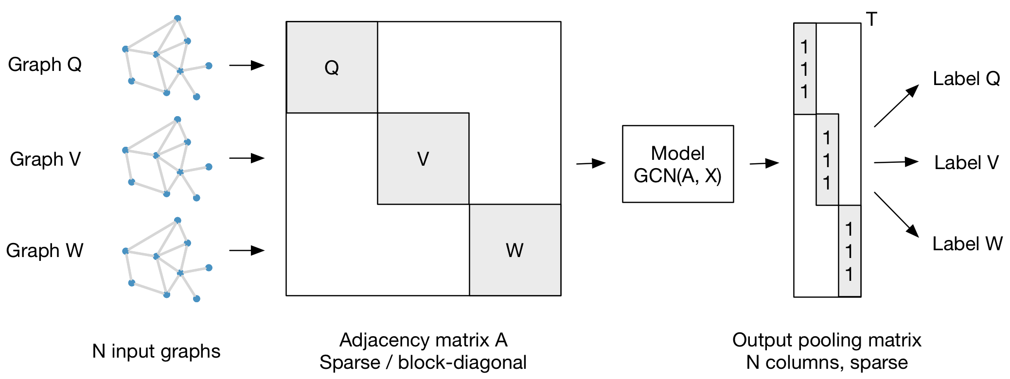
- An illustration of GCN for graph classification
- A toy application to Letter classification
- A lecture on Structured Machine Learning
Author: Romain Raveaux (romain.raveaux@univ-tours.fr)
Acknowledgement
- Datasets and functions to read data are taken from http://gmprdia.univ-lr.fr/
The lecture
The content of the is notebook is based on the following lectures : Supervised Machine Learning for structured input/output: Polytech, Tours
1. Introduction to supervised Machine Learning: A probabilistic introduction PDF
2. Connecting local models : The case of chains PDF slides
3. Connecting local models : Beyond chains and trees.PDF slides
4. Machine Learning and Graphs : Introduction and problems PDF slides
5. Graph Neural Networks. PDF slides
6. Graph Kernels. PDF slides
#!pip install networkx
#!pip install torch
#!pip install scipy
#!pip install matplotlib
Download Data
Letter Database
Graphs that represent distorted letter drawings. They consider the 15 capital letters of the Roman alphabet that consist of straight lines only (A, E, F, H, I, K, L, M, N, T, V, W, X, Y, Z). Each node is labeled with a two-dimensional attribute giving its position relative to a reference coordinate system. Edges are unlabeled. The graph database consists of a training set, a validation set, and a test set of size 750 each. Also, three levels of distortions are provided.
This dataset is part of IAM Graph Database Repository and it is also linked in the IAPR TC15 resources.
It can be considered as a TOY EXAMPLE for graph classification.
Riesen, K. and Bunke, H.: IAM Graph Database Repository for Graph Based Pattern Recognition and Machine Learning. In: da Vitora Lobo, N. et al. (Eds.), SSPR&SPR 2008, LNCS, vol. 5342, pp. 287-297, 2008.
#!wget https://iapr-tc15.greyc.fr/IAM/Letter.zip
#!unzip Letter.zip
Prepare data reader
IAM graphs are provided as a GXL file:
<gxl>
  <graph id="GRAPH_ID" edgeids="false" edgemode="undirected">
    <node id="_0">
      <attr name="x">
        <float>0.812867</float>
      </attr>
      <attr name="y">
        <float>0.630453</float>
      </attr>
    </node>
    ...
    <node id="_N">
      ...
    </node>
    <edge from="_0" to="_1"/>
    ...
    <edge from="_M" to="_N"/>
  </graph>
</gxl>import numpy as np
import xml.etree.ElementTree as ET
import networkx as nx
import torch
def read_letters(file):
"""Parse GXL file and returns a networkx graph
"""
tree_gxl = ET.parse(file)
root_gxl = tree_gxl.getroot()
node_label = {}
node_id = []
# Parse nodes
for i, node in enumerate(root_gxl.iter('node')):
node_id += [node.get('id')]
for attr in node.iter('attr'):
if (attr.get('name') == 'x'):
x = float(attr.find('float').text)
elif (attr.get('name') == 'y'):
y = float(attr.find('float').text)
node_label[i] = [x, y]
node_id = np.array(node_id)
# Create adjacency matrix
am = np.zeros((len(node_id), len(node_id)))
for edge in root_gxl.iter('edge'):
s = np.where(node_id==edge.get('from'))[0][0]
t = np.where(node_id==edge.get('to'))[0][0]
# Undirected Graph
am[s,t] = 1
am[t,s] = 1
# Create the networkx graph
G = nx.from_numpy_matrix(am)
nx.set_node_attributes(G, node_label, 'position')
return G
Load Data with NetworkX
import os

# Select distortion [LOW, MED, HIGH]
distortion = 'LOW'

# Select letter [A, E, F, H, I, K, L, M, N, T, V, W, X, Y, Z]
letter = 'K'

# Select id [0-149]
id=100

# Read the graph and draw it using networkx tools
G = read_letters(os.path.join('Letter', distortion, letter+'P1_'+ str(id).zfill(4) +'.gxl'))
nx.draw(G, pos=dict(G.nodes(data='position')))

Define dataset
Dataset Division
The dataset is divided by means of CXL files in train, validation and test with the correspondance filename and class:
<GraphCollection>
  <fingerprints base="/scratch/mneuhaus/progs/letter-database/automatic/0.1" classmodel="henry5" count="750">
    <print file="AP1_0100.gxl" class="A"/>
    ...
    <print file="ZP1_0149.gxl" class="Z"/>
  </fingerprints>
</GraphCollection>def getFileList(file_path):
"""Parse CXL file and returns the corresponding file list and class
"""
elements, classes = [], []
tree = ET.parse(file_path)
root = tree.getroot()
for child in root:
for sec_child in child:
if sec_child.tag == 'print':
elements += [sec_child.attrib['file']]
classes += sec_child.attrib['class']
return elements, classes
Define Dataset Class
Pytorch provides an abstract class representig a dataset, torch.utils.data.Dataset. We need to override two methods:
__len__so thatlen(dataset)returns the size of the dataset.__getitem__to support the indexing such thatdataset[i]can be used to get i-th sample
import torch.utils.data as data
from torch.utils.data import DataLoader

class Letters(data.Dataset):
  def __init__(self, root_path, file_list):
    self.root = root_path
    self.file_list = file_list

    # List of files and corresponding labels
    self.graphs, self.labels = getFileList(os.path.join(self.root, self.file_list))

    # Labels to numeric value
    self.unique_labels = np.unique(self.labels)
    self.num_classes = len(self.unique_labels)

    self.labels = [np.where(target == self.unique_labels)[0][0]
                   for target in self.labels]


  def __getitem__(self, index):
    # Read the graph and label
    g = read_letters(os.path.join(self.root, self.graphs[index]))
    target = self.labels[index]

    nodelist, nodes = map(list, zip(*g.nodes(data='position')))

    nodes = np.array(nodes)
    edges = np.array(nx.adjacency_matrix(g, nodelist=nodelist).todense())

    return nodes, edges, target

  def label2class(self, label):
    # Converts the numeric label to the corresponding string
    return self.unique_labels[label]

  def __len__(self):
    # Subset length
    return len(self.labels)


# Define the corresponding subsets for train, validation and test.
trainset = Letters(os.path.join('Letter', distortion), 'train.cxl')
validset = Letters(os.path.join('Letter', distortion), 'validation.cxl')
testset = Letters(os.path.join('Letter', distortion), 'test.cxl')

print(len(trainset.labels))
print((trainset.labels[100]))
print(len(trainset.graphs))
print((trainset.graphs[0]))
print((trainset.unique_labels))
print((trainset.num_classes))

print(len(validset.labels))
print(len(testset.labels))

print(trainset.__getitem__(100)[0])
print(trainset.__getitem__(100)[1])
print(trainset.__getitem__(100)[2])
Prepare DataLoader
torch.utils.data.DataLoader is an iterator which provides:
- Data batching
- Shuffling the data
- Parallel data loading
In our specific case, we need to deal with graphs of many sizes.
from scipy.linalg import block_diag

def collate(samples):
    # The input `samples` is a list of pairs
    #  (graph, label).
    batched_nodes, batched_edges, labels = map(list, zip(*samples))

    graph_shape = list(map(lambda g: g.shape[0], batched_nodes))

    # Return Node features, adjacency matrix, graph size and labels
    return  torch.tensor(np.concatenate(batched_nodes, axis=0)).float(), \
            torch.tensor(block_diag(*batched_edges)).float(), \
            torch.tensor(graph_shape), \
            torch.tensor(labels)

# Define the three dataloaders. Train data will be shuffled at each epoch
train_loader = DataLoader(trainset, batch_size=32, shuffle=True,
                         collate_fn=collate)
valid_loader = DataLoader(validset, batch_size=32, collate_fn=collate)
test_loader = DataLoader(testset, batch_size=32, collate_fn=collate)
Define Model
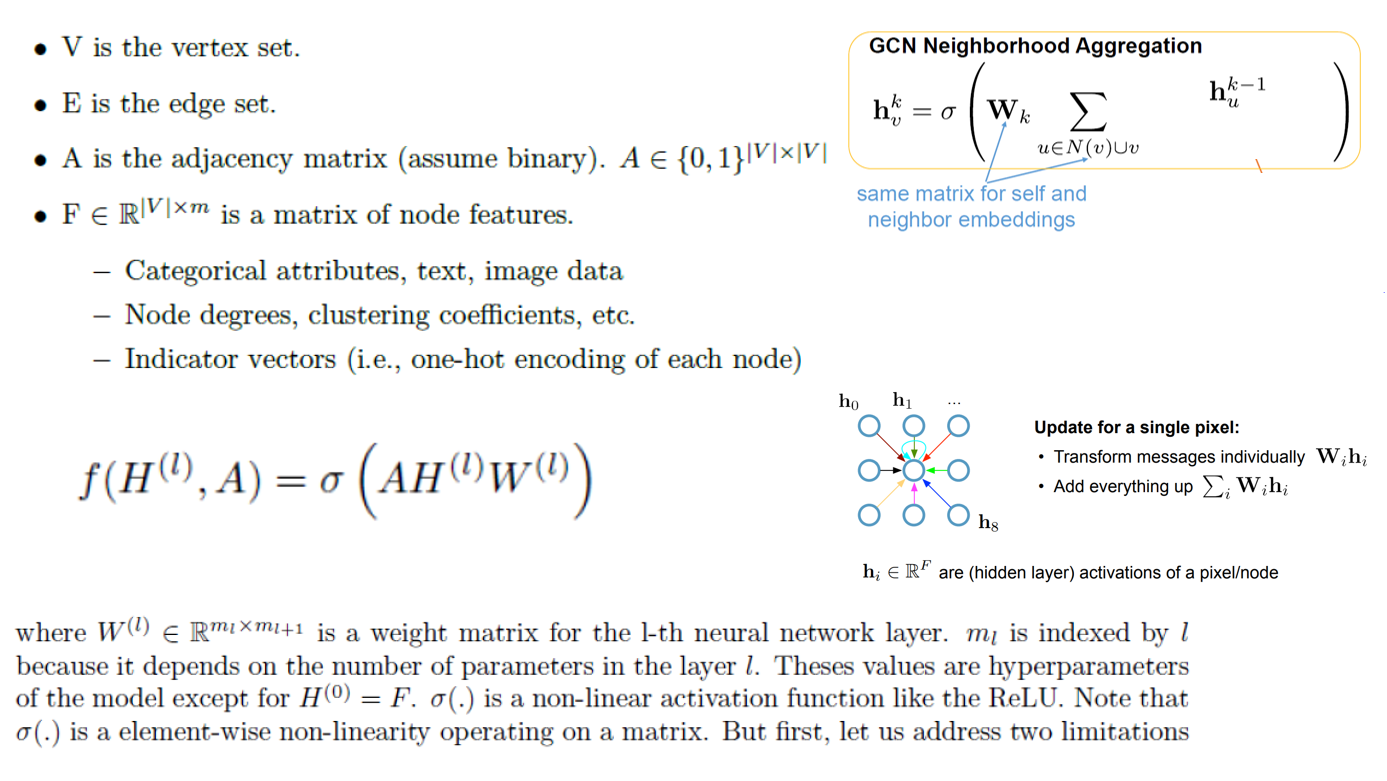
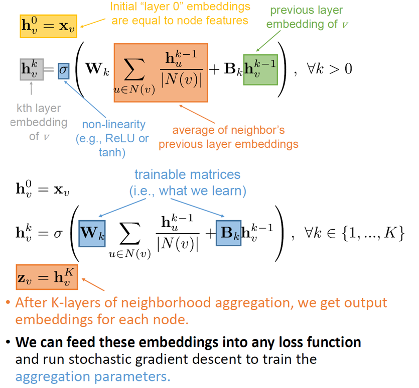
Firstly, we have to define a Graph Convolution layer
Graph Convolution
import torch
import torch.nn as nn

class GraphConvolution(nn.Module):
  """
    Simple graph convolution
  """

  def __init__(self, in_features, out_features, bias=True, batchnorm=False):
    super(GraphConvolution, self).__init__()
    self.in_features = in_features
    self.out_features = out_features
    self.bias = bias
    self.fc = nn.Linear(self.in_features, self.out_features, bias=self.bias)

    self.batchnorm = batchnorm


  #H are node features for all graphs batch
  #W are adjacency matrix for all graphs batch
  # GraphConv = AHW
  def forward(self, H, A):
    output = torch.matmul(A, H)
    #FC is just a linear function input multiplied by the paramaters W
    output = self.fc(output)

    return output
Define Model
import torch.nn.functional as F
# A Simple model with 2 graph conv layers and one linear layer for classification
# activation function are ReLus
class Net(nn.Module):
  def __init__(self, in_dim, hidden_dim, n_classes):
    super(Net, self).__init__()
    self.layers = nn.ModuleList([
        GraphConvolution(in_dim, hidden_dim),
        GraphConvolution(hidden_dim, hidden_dim)])
    self.classify = nn.Linear(hidden_dim, n_classes)

  def forward(self, h, adj, gs):
    # Add self connections to the adjacency matrix
    id = torch.eye(h.shape[0])
    m_adj=id+adj
    for conv in self.layers:
      h = F.relu(conv(h, m_adj))


    # Average the nodes
    #here we make the mean of the all the node embedding by graph
    #we do that to obtain a single vector by graph
    #we do that for classification purpose
    count=0
    hg=torch.zeros((gs.shape[0],h.shape[1]))
    for i in range(0,gs.shape[0]):
        hg[i]=h[count:count+gs[i]].mean(axis=0)
        count=count+gs[i]

    return self.classify(hg)
Training setup
import torch.optim as optim

model = Net(2, 256, trainset.num_classes)
loss_func = nn.CrossEntropyLoss()
optimizer = optim.Adam(model.parameters(), lr=0.01)
model.train()


epoch_losses = []
for epoch in range(20):
  epoch_loss = 0
  for iter, (bn, be, gs, label) in enumerate(train_loader):
    prediction = model(bn, be, gs)
    loss = loss_func(prediction, label)
    optimizer.zero_grad()
    loss.backward()
    optimizer.step()
    epoch_loss += loss.detach().item()
  epoch_loss /= (iter + 1)
  print('Epoch {}, loss {:.4f}'.format(epoch, epoch_loss))
  epoch_losses.append(epoch_loss)
Evaluation
def accuracy(output, target):
  """Accuacy given a logit vector output and a target class
  """
  _, pred = output.topk(1)
  pred = pred.squeeze()
  correct = pred == target
  correct = correct.float()
  return correct.sum() * 100.0 / correct.shape[0]


model.eval()
acc = 0
with torch.no_grad():
  for iter, (bn, be, gs, label) in enumerate(test_loader):
    prediction = model(bn, be, gs)
    acc += accuracy(prediction, label) * label.shape[0]
acc = acc/len(testset)

print('Test accuracy {:.4f}'.format(acc))
Plot results
from random import randrange
import matplotlib.pyplot as plt
for i in range(10):
  index = randrange(len(testset))
  nod, edg, label = testset[index]
  nodes, edges, gs = torch.from_numpy(nod).float(), torch.from_numpy(edg).float(), torch.tensor(nod.shape[0]).unsqueeze(0)
  if torch.cuda.is_available():
    nodes, edges, gs = nodes.cuda(), edges.cuda(), gs.cuda()
  pred = model(nodes, edges, gs)
  _, pred = pred.topk(1)

  G = nx.from_numpy_matrix(edg)
  plt.figure(i)
  position = {k: v for k, v in enumerate(nod)}
  nx.draw(G, pos=position, arrows=False)
  plt.show()
  print('Label {} {}; Prediction {} {}'.format(label, testset.label2class(label), pred.item(), testset.label2class(pred.item())))


To do by the student
import torch
import torch.nn as nn

class GraphConvolution(nn.Module):
  """
    Simple graph convolution
  """

  def __init__(self, in_features, out_features, bias=True, batchnorm=False):
    super(GraphConvolution, self).__init__()
    self.in_features = in_features
    self.out_features = out_features
    self.bias = bias
    self.fc = nn.Linear(3*self.in_features, self.out_features, bias=self.bias)

    self.batchnorm = batchnorm


  #x are node features for all graphs batch
  #W are adjacency matrix for all graphs batch
  # GraphConv = AHW
  def forward(self, H, A):
    res = torch.zeros((H.shape[0],self.in_features*3))

    output1 = torch.matmul(A[0], H)
    res[:,0:self.in_features]=output1

    output2 = torch.matmul(A[1], H)
    degree=A[1].sum(axis=0)
    deg=torch.zeros((H.shape[0],self.in_features))
    deg[:,0]=degree
    deg[:,1]=degree
    deg=deg+1
    output2=torch.div(output2,deg)
    res[:,self.in_features:2*self.in_features]=output2

    output3 = torch.matmul(A[2], H)
    output3=torch.div(output3,deg)
    res[:,2*self.in_features:3*self.in_features]=output3

    #FC is just a linear function input multiplied by the paramaters W
    output = self.fc(res)

    return output
import torch.nn.functional as F
# A Simple model with 2 graph conv layers and one linear layer for classification
# activation function are ReLus
class Net(nn.Module):
  def __init__(self, in_dim, hidden_dim, n_classes):
    super(Net, self).__init__()
    self.layers = nn.ModuleList([
        GraphConvolution(in_dim, hidden_dim),
        GraphConvolution(hidden_dim, hidden_dim)])
    self.classify = nn.Linear(hidden_dim, n_classes)

  def forward(self, h, adj, gs):
    # Add self connections to the adjacency matrix
    id = torch.eye(h.shape[0])
    adj2=torch.pow(adj,2)
    for conv in self.layers:
      h = F.relu(conv(h, [id,adj,adj2]))


    # Average the nodes
    #here we make the mean of the all the node embedding by graph
    #we do that to obtain a single vector by graph
    #we do that for classification purpose
    count=0
    hg=torch.zeros((gs.shape[0],h.shape[1]))
    for i in range(0,gs.shape[0]):
        hg[i]=h[count:count+gs[i]].mean(axis=0)
        count=count+gs[i]

    return self.classify(hg)
import torch.optim as optim

model = Net(2, 256, trainset.num_classes)
loss_func = nn.CrossEntropyLoss()
optimizer = optim.Adam(model.parameters(), lr=0.01)
model.train()


epoch_losses = []
for epoch in range(20):
  epoch_loss = 0
  for iter, (bn, be, gs, label) in enumerate(train_loader):
    prediction = model(bn, be, gs)
    loss = loss_func(prediction, label)
    optimizer.zero_grad()
    loss.backward()
    optimizer.step()
    epoch_loss += loss.detach().item()
  epoch_loss /= (iter + 1)
  print('Epoch {}, loss {:.4f}'.format(epoch, epoch_loss))
  epoch_losses.append(epoch_loss)
def accuracy(output, target):
  """Accuacy given a logit vector output and a target class
  """
  _, pred = output.topk(1)
  pred = pred.squeeze()
  correct = pred == target
  correct = correct.float()
  return correct.sum() * 100.0 / correct.shape[0]


model.eval()
acc = 0
with torch.no_grad():
  for iter, (bn, be, gs, label) in enumerate(test_loader):
    prediction = model(bn, be, gs)
    acc += accuracy(prediction, label) * label.shape[0]
acc = acc/len(testset)

print('Test accuracy {:.4f}'.format(acc))
Plot results
from random import randrange
import matplotlib.pyplot as plt
for i in range(10):
  index = randrange(len(testset))
  nod, edg, label = testset[index]
  nodes, edges, gs = torch.from_numpy(nod).float(), torch.from_numpy(edg).float(), torch.tensor(nod.shape[0]).unsqueeze(0)
  if torch.cuda.is_available():
    nodes, edges, gs = nodes.cuda(), edges.cuda(), gs.cuda()
  pred = model(nodes, edges, gs)
  _, pred = pred.topk(1)

  G = nx.from_numpy_matrix(edg)
  plt.figure(i)
  position = {k: v for k, v in enumerate(nod)}
  nx.draw(G, pos=position, arrows=False)
  plt.show()
  print('Label {} {}; Prediction {} {}'.format(label, testset.label2class(label), pred.item(), testset.label2class(pred.item())))


